Monte CarloA talk and live coding session on probabilistic simulation: from estimating π with random dots to simulating a stock portfolio the way banks do.
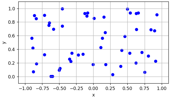
Throw enough random darts and π falls out.
Scatter points uniformly in a square, count how many land inside the quarter circle, multiply the ratio by four. The more points, the closer to π. Same trick, bigger question: replace the square with a market model and the ratio with a distribution of outcomes.
# live demo 1 · π from random points
import numpy as np
N = 1_000_000
x, y = np.random.rand(2, N)          # uniform in [0, 1)²
inside = (x**2 + y**2 <= 1).sum()
pi = 4 * inside / N                 # → 3.1416…, error ~ 1/√N
Every value equally likely. Fine for darts, wrong for markets.
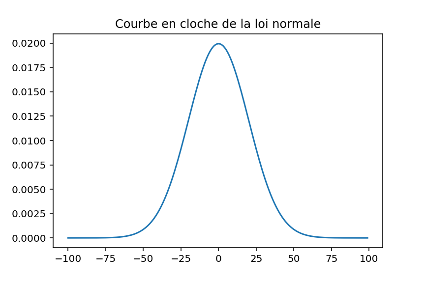
Bell curve. Most daily moves are small; extremes are rare. The standard model, and its blind spot.
Rare events happen far more than the bell predicts. Flash crashes live here.
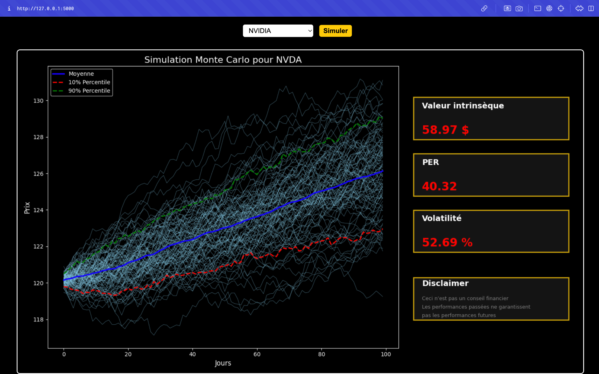
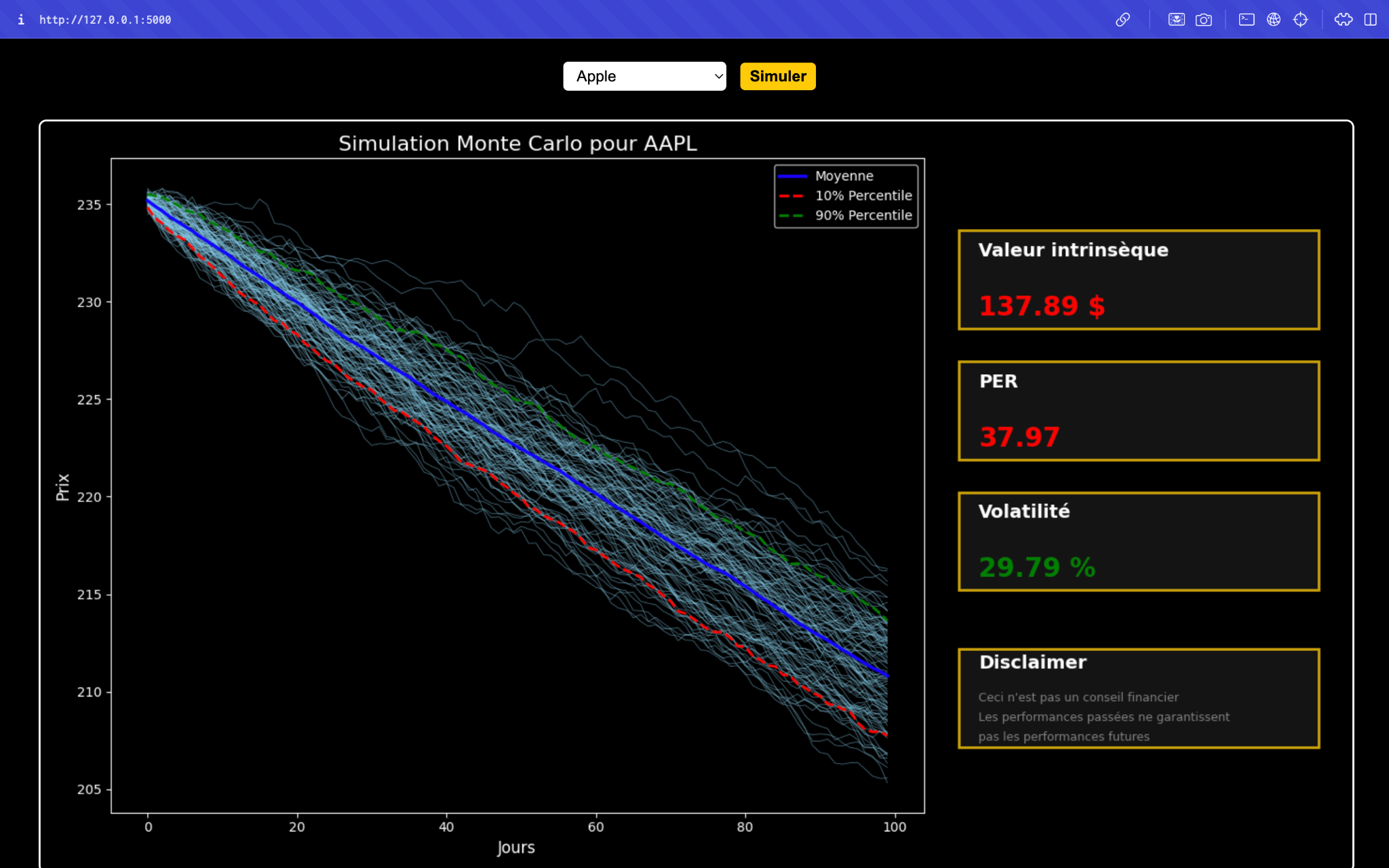
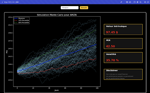
Feed a portfolio’s historical mean and volatility into thousands of random walks and read the result as a range, not a number: median outcome, best and worst percentiles, probability of loss. This is what the risk desks of the big banks run every night.
# live demo 2 · portfolio paths
mu, sigma = returns.mean(), returns.std()   # daily, from history
days, paths = 252, 10_000
shocks = np.random.normal(mu, sigma, (days, paths))
# swap for a Student-t to get fat tails:
# shocks = mu + sigma * np.random.standard_t(3, size=(days, paths)) / np.sqrt(3)
value = start * np.cumprod(1 + shocks, axis=0)
p5, p50, p95 = np.percentile(value[-1], [5, 50, 95])
loss_prob = (value[-1] < start).mean()
- Drift and volatility come from history; the randomness is the model’s honesty about what it doesn’t know.
- 10,000 paths, 252 trading days: enough that the percentiles stop moving between runs.
- The distribution is a switch. Normal to Student-t changes the 5th percentile far more than the median. That switch is the whole talk.
Automation begins on the trading floor.
Paris closes the pit.
High-frequency trading, big data, and a market that fell 9 % in minutes.
Quant tools reach everyone.
Four of five household names fell. The room guessed mostly up. That was the point of the disclaimer slide.